Tutorial
Sanepic Tutorial -- The Polaris field
In this tutorial, we will produce an optimal map of Polaris, a galactic field with cirrus emission on all scales. In this case, the data have been optained by the Herschel/SPIRE instrument. We will use a single computer with large local disk and multiple cores in order to speed up the calculations.
Install SANEPIC
You will first download the source code of SANEPIC and install it quickly (assuming you have all the required librairies) with :
> gunzip sanepic-x.x.tar.gz | tar xvf -
> cd sanepic-x.x
> ./configure --prefix=$HOME --enable-parabolo
> make install
The code is compiled using the parabolo option, with is better suited in our case as we only have 2 scans, but lots of bolometers. It is now installed in our $HOME/bin& $HOME/libdirectories. So you should add these directory to you shell startup scripts, for e.g. in $HOME/.bashrc:
export PATH=$HOME/bin:$PATH
export LD_LIBRARY_PATH=$HOME/lib:$LD_LIBRARY_PATH
Download the Data
First download the data and input file that we will use in this tutorial. The data consist of two observations made by Herschel/SPIRE, processed with HIPE and exported to the SANEPIC data format. If you move the data files into a data subdirectory, you should end up with
SANEPIC_tutorials
├── data
│   ├── OD162_0x500022F9L_SpirePacsParallel_polaris_notdf_all_sanepic.fits.gz
│   ├── OD162_0x500022F9L_SpirePacsParallel_polaris_notdf_all_sanepic_psd.fits.gz
│   ├── OD162_0x500022FAL_SpirePacsParallel_polaris_notdf_all_sanepic.fits.gz
│   └── OD162_0x500022FAL_SpirePacsParallel_polaris_notdf_all_sanepic_psd.fits.gz
├── inputDir
│   ├── fCutFile.fcut
│   ├── listFile.list
│   ├── OD162_0x500022F9L_SpirePacsParallel_polaris_notdf_all_sanepic_PLW.bolo
│   └── OD162_0x500022FAL_SpirePacsParallel_polaris_notdf_all_sanepic_PLW.bolo
└── sanepic.ini
Running the scripts
Let start by setting up SANEPIC and extracting the needed data from the fits file :
> mpirun -n 2 sanePre_PARA_FRAME sanepic.ini
as we are only dealing with two observations, we only use 2 processes here.
sanePre :  pre processing of the data

WW - ./Output/ created
WW - ./tempDir/ created

Data Dir.        : ./data/
Input Dir.       : ./inputDir/
Temp. Dir.       : ./tempDir/
Output Dir.      : ./Output/
# of Scans       : 2

Exporting signal and flags...
Exporting positions...
Exporting header keys...

end of sanePre
Now the data are reading to be processed. We can continue by computing the map parameters and the pixel indexes for each bolometers
> mpirun -n 2 sanePos_PARA_FRAME sanepic.ini
Again, this part of SANEPIC is using only two processors.
sanePos: computation of pixel indexes


Data Dir.        : ./data/
Input Dir.       : ./inputDir/
Temp. Dir.       : ./tempDir/
Output Dir.      : ./Output/

Pixel Size       : 0.00388888888889 deg
Map Flags        : True
Gap Filling      : PROJECTED

# of Scans       : 2

Determining Map Parameters...

WW - Projections will have to be made twice, define a projection center...
WW - Nominal Projection Center :
     lon : 55.649343231546
     lat : 88.735659667811

Map Size         : 1035 x 990 pixels

Computing pixel indexes...
Pixels Indices   : 2049303
Filled Pixels    : 1123886

Computing Naïve map...
Output file      : naivMap.fits

End of sanePos
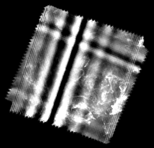
At this stage we can already have a look at the naive map produced by sanePos. Only a quick preprocessing (baselining, mild high-pass filter) is applied on the timelines, thus we see a lot of stripes/drifts in the map as the data are not corrected from the thermal drift of the telescope.
We need to invert the Noise-Noise PowerSpectra given the list of bolometer we want to use :
> mpirun -n 2 saneInv_PARA_FRAME sanepic.ini
saneInv : Inversion of the Noise-Noise PowerSpectra


Data Dir.        : ./data/
Input Dir.       : ./inputDir/
Temp. Dir.       : ./tempDir/
Output Dir.      : ./Output/

Noise Dir.       : ./data/

# of Scans       : 2
2 covariance Matrix will be inverted

Inverting Covariance Matrices...
done.

End of saneInv
Finally, we can launch the final program, performing the full gradient descent, using for example 12 processors :
> mpirun -n 12 sanePic_PARA_BOLO sanepic.ini
Beginning of sanePic : conjugate gradient descent


Data Dir.        : ./data/
Input Dir.       : ./inputDir/
Temp. Dir.       : ./tempDir/
Output Dir.      : ./Output/

Pixel Size       : 0.00388888888889 deg
Map Flags        : True
Gap Filling      : PROJECTED

Fill Gaps        : True
Simple Baseline  : will be removed (default)
Correlations     : INCLUDED in the analysis
Poly. Order      : 1
# for Apodize    : 100
HPF Freq.        : 0.000366 Hz
Sampling Freq.   : 10.016081 Hz

Write Iter. Maps : 10
Max Iter.        : 2000
Maps prefix      : optimMap

# of Scans       : 2
Map Size         : 1035 x 990 pixels


Computing Pre Conditioner...
Starting Conjugate Gradient Descent...

[...]

done.

End of sanePic
The optimal map should now be completed. You can find it under the Outputdirectory as, by default, Output/optimMap_sanePic.fits
Results
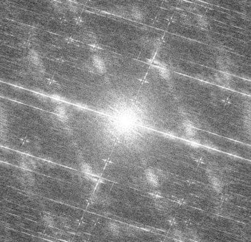
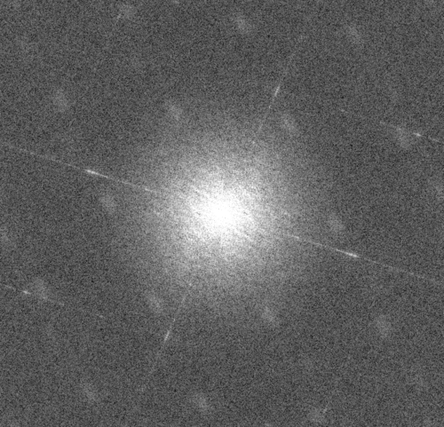
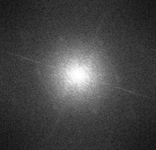
You can find, in the following gallery, a comparison between the optimal map produced by SANEPIC and the map produced by combining the two obsids fully processed by the default pipeline of HIPE including the thermal drift corrections based on the thermistors. The difference of those two maps is highlighted with an higher dynamic range. One can see that a lot of stripping is removed, as well as recovering of the large scales. This is also illustrated in the 2D FFT of the images, which clearly show the removal of the 1/f noise/drift in the case of the SANEPIC processing. All the images share the same dynamic range.
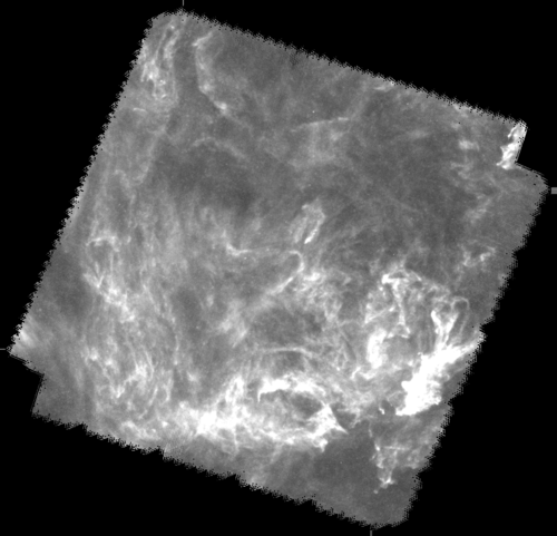
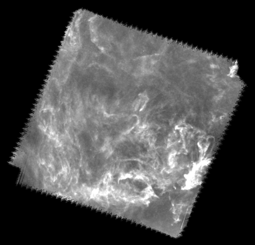
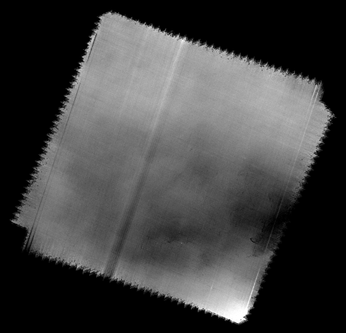
The middle column show the results obtained using the HIPE destriper in v7.2. One can see that the striped are indeed well removed from the image, but are still present, as well as a filtering of the largest scale in the image compared to SANEPIC.